| |
| Evaluators |
Plan: Methodology overview


The main purpose of this guide is to help you use institutional data to evaluate student success, and the bulk of this page will focus on unpacking quantitative causal methods. We include explanations, examples, diagrams and key considerations for each quantitative causal methodology.
However, after following the flowchart, you may have found that generating quantitative causal evidence isn’t feasible in your situation. This could be, for example, because your sample size is too small, or the outcomes you’re interested in are not meaningfully measurable in a quantitative manner. If this applies, please see our section on impact evaluation with small cohorts.
Causal evaluations (type 3)
Deciding which methods are most suitable to produce causal evidence can feel difficult. The flowchart and the following sections will help you explore which experimental or quasi-experimental methods might work for your evaluation.
Before using any specific experimental or quasi-experimental method, it is also important to consult more detailed resources. Each method comes with its own set of assumptions, requirements and considerations that will significantly impact the validity and reliability of your research findings.
TipCausal evaluation resources
TASO: Evaluating complex interventions using randomised controlled trials
Causal Inference: The Mixtape (Scott Cunningham)
Mostly Harmless Econometrics (Joshua D. Angrist & Jörn-Steffen Pischke)
Designing Randomised Trials in Health, Education and the Social Sciences (David Torgerson & Carole Torgerson)
Impact Evaluation in Practice (World Bank)
Econometrics with R (Christoph Hanck, Martin Arnold, Alexander Gerber, and Martin Schmelzer)
Causal Inference for the Brave and True (Matheus Facure Alves)
As with the flowchart, these sections adapt and build on insights from the Magenta Book, published under the Open Government Licence.
Quasi-experimental designs (QED)
Difference-in-difference
- This method estimates the effect of an intervention by comparing the difference in outcomes between those who received the intervention and those who did not, before and after the intervention took place.
- This method helps to isolate the effect of receiving the intervention from other changes over time that might affect the outcome, allowing you to control for unobserved factors.
- This method relies on the assumption that both groups would have followed similar trends in outcomes over time if the intervention wasn’t introduced (parallel trends assumption).
NoteDifference-in-difference example
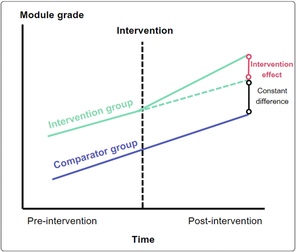
A mentoring programme is designed to improve module grades.
It is rolled out to students in one academic department, but not to students in another similar department.
The students in both departments have similar characteristics.
Prior to the intervention the trends in attainment over time were similar.
Considerations
- Difficult if there is no clear timing of the intervention.
- For the most robust evaluation, requires outcome data before, during and after the intervention.
- Identifying a suitable comparator group can be difficult.
- Parallel trends assumption can be hard to establish and may not hold true.
Regression discontinuity design
- This method estimates the effect of an intervention for which participant eligibility depends on whether an individual exceeds a threshold or cutoff (e.g. module grade).
- Individuals on either side of the cutoff are assumed to be similar, except for whether they received the intervention or not.
- By comparing individuals just below the cutoff (and did not receive intervention) to those just above (and did receive the intervention), any difference in outcomes can be attributed to the intervention, providing causal evidence.
NoteRegression discontinuity design example
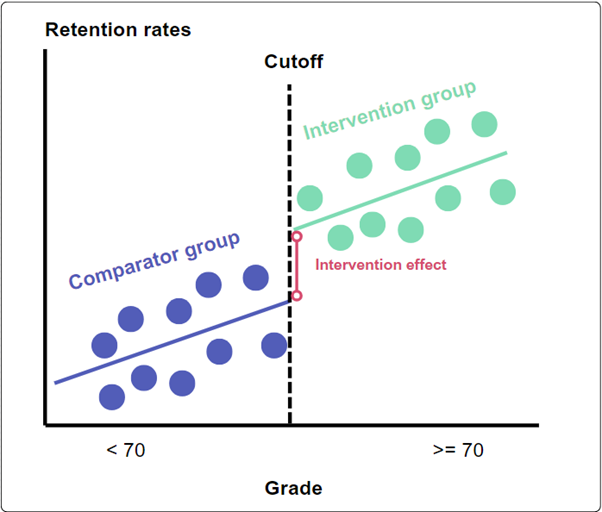
A bursary is given to disadvantaged students achieving a final grade of 70 or higher at the end of their first year, aiming to increase retention.
Retention rates of disadvantaged students who would have been eligible, but scored 69 (and a little below), are compared with students who scored 70 (and a little above) and received the bursary.
The comparison groups are clearly and objectively defined by the cutoff.
Considerations
- Conclusions may not apply to those further from the cutoff
- Accurate estimation requires a large amount of data close to the cutoff.
Instrumental variables
- This method can be used when there is an external factor (the instrument) that influences whether someone participates in the intervention, but is not directly linked to the outcome being studied.
- A good instrumental variable is exogenous; that is the instrumental variable must affect the likelihood of taking part in the intervention but be unrelated to the outcome, other than through the intervention itself.
- This method deals with hidden biases (such as motivation) and can address unobserved confounding variables. By comparing the outcomes of those influenced by the instrument to join the intervention to those who are not, the effect of the intervention can be determined.
NoteInstrumental variables example
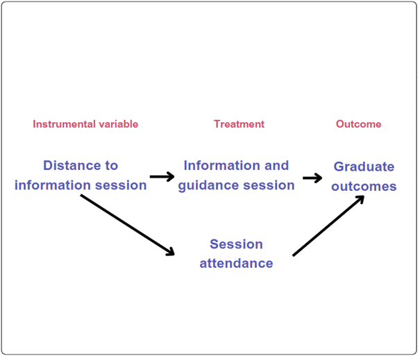
An information and guidance session aims to improve graduate outcomes (e.g. employment).
The distance a student would have to travel to the session location might be a good instrument that could be both relevant to participation in the session and unrelated (external or exogenous) to the session outcomes could be the distance to the session location:
Relevant: The distance between a student’s residence and the session location could influence their chances of attending.
Unrelated: The distance a student travels to the session is unlikely to directly affect graduate outcomes. It influences outcomes primarily through its effect on session attendance.
Considerations
- Finding a valid instrument is hard: many factors will have some association with outcomes.
- Potential bias if the instrumental variable influences the outcome by a means unrelated to the intervention (i.e., it is not perfectly exogenous).
Matching methods
- These methods can be used to create a comparison group by matching individuals from the population who do not receive an intervention with individuals who do using characteristics (such as grades, entry route, gender, ethnicity) that could influence both the likelihood of receiving the intervention and the outcomes of interest.
- The comparison group and intervention group will be similar based on those key characteristics. This creates pairs or groups that are comparable, except for the intervention.
NoteMatching methods example
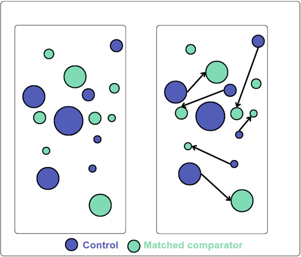
A new online tutoring programme for first-year students struggling with quantitative skills is introduced.
To evaluate its impact on grades, students who receive the programme are matched with similar students who do not, based on their entry route to higher education, prior module marks, and VLE engagement, creating comparable groups.
The grades in these groups are then compared.
This approach is intuitive and easy to understand, and can be more powerful when paired with a difference-in-difference method.
Considerations
- Matching can only control for observed variables; any differences in unobserved variables can bias the results.
- Heavily relies on the availability and quality of data on relevant covariates.
Interrupted time-series analysis
- This method can be used when an intervention takes place in the whole population of interest and the outcome measure is known over a period of time before and after an intervention (the interruption).
- The effects of an intervention are evaluated by obtaining outcome measures at several points before and after an intervention is introduced, allowing the change in level and trend of outcomes to be compared.
NoteInterrupted time series example
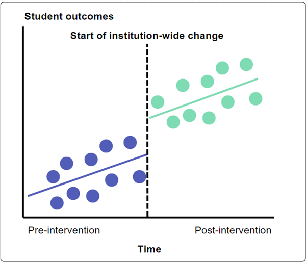
A HEP introduces an institution-wide change in mental health and wellbeing support, which includes support for all students at key transition points and ‘mental health champions’ on every course.
Student outcomes across the HEP - such as wellbeing, engagement and attainment - before and after the change was introduced are compared.
Considerations
- Requires extensive data before and after the intervention (whole-provider change) comes in.
- Confidence in the causal impact of the intervention can be higher if there are no other changes occurring around the time of the intervention which could also affect the outcome. Consequently, unexpected events that occur around the time of the intervention may influence outcomes and confound the results.
- If any changes in outcome and/or its trend do not match the intervention’s timing, then it is hard to support a cause-and-effect relationship.
Synthetic control methods
- Similar to a difference-in-difference design but uses data prior to the intervention to construct a ‘synthetic clone’ of a group receiving a particular intervention through the weighted average of groups not receiving the intervention.
- Differences between the performance after the intervention begins between the intervention group and its synthetic clone may be used as evidence that the intervention has had an effect. Most commonly applied to interventions applied at an area or group level.
- One key strength of synthetic controls is that they can offer a relevant comparison when no other comparators exist.
NoteSynthetic control methods example
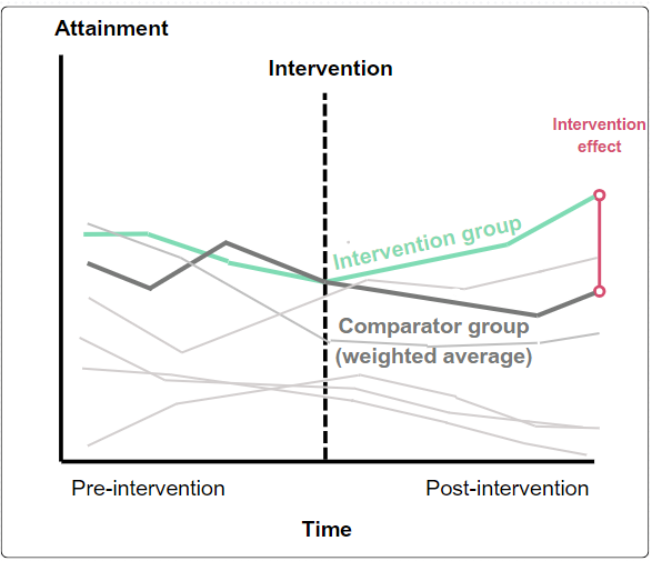
A module within an academic department is trialling changes in assessments to see if this supports wellbeing and attainment.
A synthetic control is created using a weighted average of student assessments from other modules.
The outcomes of this synthetic control prior to the change in assessment broadly match those of students on the reformed module.
The intervention effect can be inferred from the difference in outcomes at the end of the trial period.
Considerations
- Only viable when it can be demonstrated that there was a relationship between the behaviour of the intervention and comparator groups in the period before the intervention.
- Developing a synthetic control requires extensive historical data: suitable when large volumes of secondary data are already available.
- Can be used on small sample sizes.
Randomised controlled trials (RCTs)
Individual RCT
- In a two-arm RCT individuals are randomly assigned to one of two groups. These two groups are usually the control group - who receive either no intervention orbusiness as usual - and the intervention group (sometimes referred to as the treatment group) who do receive the intervention.
- Random assignment helps ensure that the individuals in each group are similar in all ways except for the intervention they receive.
- Any difference in outcomes between the groups is the intervention’s real effect.
- RCTs (with implementation and process evaluation) are often considered the strongest way of testing the effectiveness of an intervention.
NoteIndividual RCT example
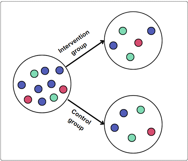
A learning analytics system flags students who have low levels of engagement.
Each student who is flagged is randomly assigned to receive either an email, or an email plus a phone call.
Considerations
- Running an RCT can be expensive and take a lot of time.
- Sometimes it is not possible or ethical to withhold the intervention from those who might benefit from it, making RCTs impractical; though see Waitlist or Stepped-wedge RCTs.
- RCTs are generally more ethical where there is no clear consensus about the effect of the intervention.
- The generalisability may be limited if the study setting is very controlled.
Cluster RCT
- In a two-arm cluster RCT, groups (clusters) of individuals are randomly assigned to one of two groups.
- These two groups are usually the control group - who receive either no intervention or business as usual - and the intervention group (sometimes referred to as the treatment group) who do receive the intervention.
- Cluster RCTs are used when interventions are delivered to pre-existing groups (e.g. students on a module) and individual random allocation is not possible.
- Delivering interventions to entire groups can reduce the risk of control group participants being exposed to the intervention (spillover effects).
NoteCluster RCT example
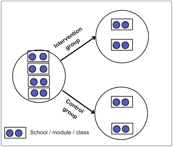
- Participants are randomly assigned to receive a change in assessment type by academic school, with Business School and School of Social Sciences receiving the intervention, while School of Engineering and Mathematics and School of Life Sciences do not receive the intervention.
Considerations
- If the clusters themselves are not randomly selected, there is a potential for selection bias.
- Cluster RCTs often require larger samples than individual-level RCTs to achieve similar levels of statistical confidence, making them more resource-intensive.
Waitlist or stepped-wedge RCT
- These RCT methods are suitable when it is not ethical or desirable to permanently withhold an intervention. All participants eventually receive the intervention, which is especially important for interventions which we have strong reason to believe will be beneficial.
- Can be easier to implement than traditional RCTs.
- Waitlist RCT:
- Participants are randomly assigned to either receive the intervention immediately or be placed on a waiting list (control group) and receive the intervention after a delay.
- Stepped-wedge RCT:
- All participants or clusters eventually receive the intervention, but the start times are randomly assigned so the intervention is rolled out in steps or phases.
- A stepped-wedge RCT can be thought of like a waitlist RCT with more than one delay period.
NoteWaitlist RCT example
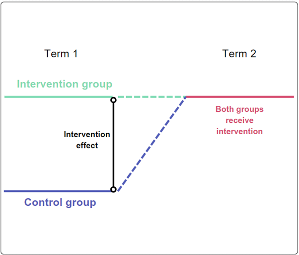
Wellbeing intervention targeted at STEM students has only 100 places per term, but 200 eligible students.
100 students are randomly assigned to receive the intervention in term 1, while the other 100 are assigned to a waitlist control group.
The outcomes for both groups are measured at the end of term 1.
Then in term 2, the waitlist control group receives the intervention.
Considerations
- If the intervention’s effectiveness changes over time, the design might not capture this accurately.
- As everyone ultimately receives the intervention, long-term outcomes cannot be measured.
Correlational evaluations (type 2)
Type 2 evidence might tell us that students who take part in an activity have better outcomes than other students, for example, we might compare attainment for students who take part in an activity versus those who don’t.
This kind of evidence allows us to understand if there is an association/correlation between taking part in an activity and better outcomes. However, it cannot tell us whether the activity actually causes the improvement or if other factors are responsible.
The same techniques used in identifying the gaps in the first place - visually or with inferential statistics (t-tests, ANOVA, regression) - can be used to monitor their progression once an intervention is in place.
Theory-based evaluation
Impact evaluation is important but can be challenging. TASO promotes the use of rigorous experimental and quasi-experimental methodologies as these are often the best way to determine causal inference. However, sometimes these types of impact evaluation raise challenges:
- They are effective in describing a causal link between an intervention and an outcome, but less good at explaining the mechanisms that cause the impact or the conditions under which an impact will occur.
- They require a reasonably large number of cases that can be divided into two or more groups. Cases may be individual students or groups that contain individuals, such as classrooms, schools or neighbourhoods.
- Most types of experiment – and some types of quasi-experiment – require evaluators to be able to change or influence (manipulate) the programme or intervention that is being evaluated. However, this can be difficult or even impossible, perhaps because a programme or intervention is already being delivered and the participants already confirmed or because there are concerns about evaluators influencing eligibility criteria.
- Experimental and quasi-experimental evaluation methodologies can sometimes struggle to account for the complexity of programmes implemented within multifaceted systems where the relationship between the programme/intervention and outcome is not straightforward.
An alternative group of impact evaluation methodologies, sometimes referred to as ‘theory-based methodologies,’ can address some of these challenges:
- They only need a small number of cases or even a single case. The case is understood to be a complex entity in which multiple causes interact. Cases could be individual students or groups of people, such as a class or a school. This can be helpful when a programme or intervention is designed for a small cohort or is being piloted with a small cohort.
- They can ‘unpick’ relationships between causal factors that act together to produce outcomes. In theory-based evaluation methodologies, multiple causes are recognised and the focus of the impact evaluation switches from simple attribution to understanding the contribution of an intervention to a particular outcome. This can be helpful when services are implemented within complex systems.
- They can work with emergent interventions where experimentation and adaptation are ongoing. Generally, experiments and quasi-experiments require a programme or intervention to be fixed before an impact evaluation can be performed. Theory-based methodologies can, in some instances, be deployed in interventions that are still changing and developing.
- They can sometimes be applied retrospectively. Most experiments and some quasi-experiments need to be implemented at the start of the programme or intervention. Some theory-based methodologies can be used retrospectively on programmes or interventions that have finished.
TipResources for impact evaluation with small cohorts
TASO has some guidance for theory-based evaluation.
Implementation and process evaluation
This type of evaluation provides information about how best to revise and improve activities. It can be used to assess whether the initiative, analysis and underlying assumption(s) are being implemented as intended. It is often helpful for pilot projects and new services and schemes. Implementation and process evaluation can also be used to monitor the progress and delivery of ongoing initiatives. IPE can help you:
- evaluate whether an intervention or programme was implemented as intended
- identify the elements of an intervention or programme that are necessary to produce the intended effects (outcomes)
- establish whether the assumption(s) and mechanisms underpinning the intervention’s theory of change hold true.
TipImplementation and process evaluation resources
TASO has published several resources to support the sector in conducting rigorous IPE:
IPE guidance - provides an introduction to IPE and step-by-step process for completing an IPE
IPE framework - provides a summary of the TASO IPE framework and step-by-step approach to implementing the guidance
Case study - an illustrative example of an IPE protocol for an access intervention
IPE protocol template - to guide the sector in designing and developing their own IPEs
IPE reporting template - to guide the sector in structuring and developing their own IPE reports